Processing Industrial Telemetry at Scale with AWS Batch, Spot, and Bedrock

A fictional but realistic scenario: a global industrial operator runs thousands of manufacturing sites around the world. Each site streams high-frequency sensor telemetry - vibration, bearing temperatures, oil pressure, coolant flow, motor current, fault flags - from 24 channels sampled at 1 kHz. At the end of each monitoring window, a parquet file lands in S3 for each site. A few thousand files, each a few GB, each with millions of rows. The pipeline needs to ingest them, run real signal processing (rolling anomaly detection, FFT spectral analysis, fault flag decoding), and generate a per-site incident report so the reliability team knows where to send a technician.

This is exactly the kind of workload AWS Batch was built for.

It's also the kind of workload where EC2 Spot can cut your compute bill by 70-90%. Add Amazon Bedrock for LLM-based incident reports on each file, and you've got a complete predictive maintenance pipeline where the core architecture stays the same whether you're processing ten sites or ten thousand. (Real scaling always brings quota adjustments, timeout tuning, and cost controls along with it, but the code and infrastructure pattern here don't have to change.)

In this post I'll walk through how I built this end-to-end demo using Terraform, Python 3.14, AWS Batch with Spot, scipy for the signal processing, Amazon Bedrock (Nova Pro by default), and a small React 19 + Vite 7 frontend so you can browse the incident reports from your laptop. The full code is on GitHub and you can deploy it into your own account in about 10 minutes. Everything is in the repo on GitHub.

Why AWS Batch fits this workload

If you're new to AWS Batch, here's the elevator pitch: it's a managed service that runs containerized batch jobs on EC2 (or Fargate). The compute environments scale automatically based on queue depth. You define a job, you submit it, Batch figures out how much compute to spin up, runs your container, and then scales back to zero when there's nothing to do. You only pay for the compute while jobs are running.

That last bit matters. Industrial telemetry arrives in batches at predictable intervals (say, once per hour or once per shift). Between runs, we want zero compute cost. With min_vcpus = 0, Batch has zero compute instances running between batches - no EC2 charges at all. (The supporting infrastructure like the NAT gateway and Bedrock VPC endpoint still has hourly charges; more on that in the cost section.) When the next set of files lands, Batch spins up instances on demand, processes everything, and tears the compute back down.

Each file in this demo contains 24 float64 sensor channels. The container runs real signal processing: rolling-window z-score anomaly detection, FFT spectral analysis on vibration channels using scipy's Welch method, and decoding of a fault-flag bitfield.

The analysis I've written here is deliberately modest and finishes in tens of seconds per file on 4 vCPUs with 16 GB RAM. That's fine for this demo. The point isn't that the current workload requires Batch - it's that the architecture gives you room to grow into heavier analysis without rearchitecting.

A word about Lambda

To be upfront: Lambda would work for what this demo does today. If your per-file processing is always going to be a few seconds of signal processing and an LLM call, Lambda is a perfectly reasonable choice. I picked Batch because I wanted to build an example with Batch, and because in real industrial monitoring the analysis almost never stays simple.

Here's what tends to happen over time:

• You add more sensors per site (128 channels instead of 24)
• You increase the sample rate (10 kHz instead of 1 kHz) for better fault detection
• You add envelope detection, cepstrum analysis, or order tracking on top of the FFT
• You train a small ML model on historical data and run inference per file
• You join against a database of equipment metadata or prior inspection reports
• You extend the monitoring window from 1 hour to a full shift or a full day

Any one of those changes can push a file's processing time from seconds into minutes or tens of minutes. Several of them push you past Lambda's 15-minute ceiling, its 10 GB RAM ceiling, or both.

At that point you're rebuilding the pipeline under deadline pressure. Starting with Batch means the same code and infrastructure handles the lightweight case today and the heavy case later - you just bump job_vcpus, job_memory_mib, and job_timeout_seconds in your tfvars and keep going. Add envelope detection, longer rolling windows, ML inference, or more sensor channels and that per-file time climbs, which is where Spot savings really start to add up.

Here's where Batch genuinely shines versus the alternatives when the workload has any of those characteristics:

Alternative	Where Batch wins when the workload is a good fit
Lambda	Long-running jobs (10+ minutes per file), memory over 10 GB, workloads that benefit from packing multiple tasks onto shared instances, access to GPU or specific instance families, custom AMIs
ECS/Fargate	You'd build your own scheduling, scaling, and queue logic that Batch already gives you for free
EMR / Spark	Overkill for embarrassingly parallel per-file work - this isn't a join or aggregate problem
Step Functions	Excellent for orchestration but not for the actual compute - you'd still need somewhere to run the work
EKS	You'd build everything Batch already provides, with more YAML

The Batch sweet spot is bursty, embarrassingly parallel, container-based work that benefits from spot pricing - especially where jobs are long-running, memory-heavy, or might grow into those shapes over time. Industrial telemetry is one of many workloads that starts light and gets heavier as the analysis matures.

Why Spot makes sense (and how Batch makes it easy)

EC2 Spot Instances let you use AWS's spare capacity and save up to 90% compared to on-demand pricing. The tradeoff is that AWS can reclaim those instances with two minutes of notice if they need the capacity back.

For interactive workloads or stateful systems, that tradeoff is scary. For our per-file processor, the savings are very attractive:

• Each file is processed independently. If a container dies mid-file, we just retry that file.
• Results are written to S3 after each file completes, so completed work survives interruptions.
• Batch has built-in retry policies that automatically requeue jobs that fail due to spot reclamation.
• We have an on-demand compute environment as a fallback for when spot capacity isn't available.

The on-demand fallback is the trick that makes spot safe: the job queue is configured to try the spot compute environment first, and only spill to on-demand if spot capacity isn't available. Most of the time, you pay spot prices. When AWS is having a busy day, your jobs still run.

For instance type selection, I use the optimal setting which lets Batch automatically pick from a diverse pool of instance families and sizes. optimal still works and is what the demo uses, but newer Batch environments can also use default_x86_64 or default_arm64 explicitly - optimal now maps to default_x86_64 under the hood, and AWS updates these bundles as new instance families launch in your region.

Combined with the SPOT_PRICE_CAPACITY_OPTIMIZED allocation strategy (which AWS now recommends over the older SPOT_CAPACITY_OPTIMIZED), Batch finds the cheapest spot pools that are also least likely to be interrupted.

The architecture

Here's everything that gets deployed by Terraform:

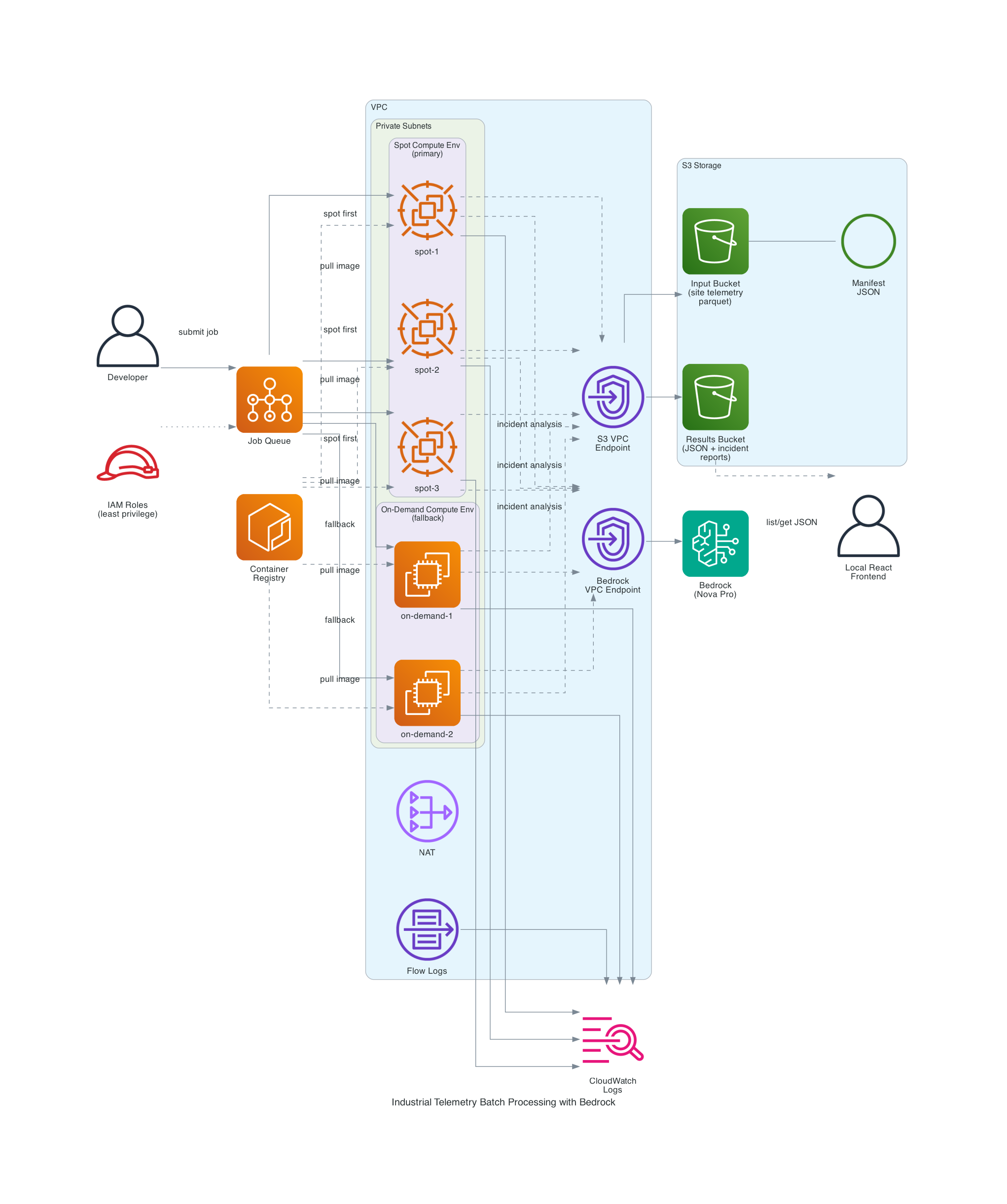
The pieces:

Component	What it does
S3 Input Bucket	Stores site telemetry parquet files and the file manifest JSON
S3 Results Bucket	Receives per-file processing results and LLM incident reports (separate bucket from input)
ECR Repository	Hosts the Python 3.14 processor container image
AWS Batch Spot CE	Primary compute - SPOT_PRICE_CAPACITY_OPTIMIZED allocation across diverse instance types
AWS Batch On-Demand CE	Fallback compute for when spot capacity isn't available
Job Queue	Routes jobs to spot first, on-demand second
Launch Template	Custom AMI support, IMDSv2 enforcement, instance/volume naming
VPC	Private subnets, NAT gateway, S3 gateway endpoint, VPC flow logs
Bedrock VPC Endpoint	Keeps LLM traffic on the private network
CloudWatch Logs	Per-container output and processing summaries
IAM Roles	Least-privilege: separate roles for ECS instance, job execution, job task, spot fleet, and Bedrock

Two things worth pointing out:

1. The S3 gateway endpoint is free and saves you NAT charges for all the parquet downloads. At multi-GB file sizes and thousands of files per run, this matters a lot.
2. The Bedrock interface endpoint keeps LLM API calls inside your VPC. It's an interface endpoint, not a gateway, so it has an hourly cost, but the traffic isolation is often worth the hourly cost in security-conscious production environments.

How the processing flow works

Step 1: The manifest

All processing starts from a manifest file in S3 - a simple JSON document that lists every parquet file to process:

{
  "version": 1,
  "bucket": "my-input-bucket",
  "prefix": "input/",
  "files": [
    {"bucket": "my-input-bucket", "key": "input/site_telemetry_00000.parquet"},
    {"bucket": "my-input-bucket", "key": "input/site_telemetry_00001.parquet"}
  ],
  "total_files": 1000
}

In my demo the data generator builds the manifest automatically when uploading the synthetic site files. In a real pipeline, you'd build it from your data ingestion system or an aws s3 ls of the input prefix.

Step 2: Submitting an array job

scripts/submit_jobs.py reads the manifest, counts the files, calculates how many array job indices to submit based on a FILES_PER_JOB setting, and submits a single AWS Batch array job with that size.

An array job is just one job submission that spawns N "child jobs" where each one gets a different AWS_BATCH_JOB_ARRAY_INDEX environment variable from 0 to N-1. This is the canonical Batch pattern for embarrassingly parallel work.

1000 files / FILES_PER_JOB=10 = 100 array indices = 100 containers
1000 files / FILES_PER_JOB=5  = 200 array indices = 200 containers
1000 files / FILES_PER_JOB=1  = 1000 array indices = 1000 containers

I can dial parallelism up or down with one environment variable.

Step 3: File partitioning inside the container

Each container that Batch spawns gets two environment variables that AWS Batch sets automatically:

• AWS_BATCH_JOB_ARRAY_INDEX - this container's index (0, 1, 2, ...)
• AWS_BATCH_JOB_ARRAY_SIZE - the total number of containers in the array

The container downloads the same manifest, then deterministically slices it based on those two variables:

def partition_files(files: list[dict]) -> list[dict]:
    total = len(files)
    chunk_size = total // ARRAY_SIZE
    remainder = total % ARRAY_SIZE

    if ARRAY_INDEX < remainder:
        start = ARRAY_INDEX * (chunk_size + 1)
        end = start + chunk_size + 1
    else:
        start = ARRAY_INDEX * chunk_size + remainder
        end = start + chunk_size

    return files[start:end]

This handles uneven divisions cleanly. Every file is processed exactly once and there's no coordination between containers.

Step 4: The signal processing pipeline

This is where the real work happens. For each assigned file, the container runs a pipeline that actually resembles production industrial monitoring code:

1. Download and column projection. The parquet file is downloaded from S3 and loaded with pyarrow using column projection - we only read the columns we need. For a 500K-row file with 24 sensor columns plus timestamps and flags, we're loading about 100 MB into memory as float64 arrays. Bump RECORDS_PER_FILE to 3_600_000 for a full-hour window at 1 kHz and that climbs to around 700 MB per file, which is where the 16 GB memory allocation on the job definition starts to matter.

2. Per-sensor statistics. Global min, max, mean, and std for all 24 channels.

3. Rolling-window anomaly detection. For every sensor, compute a 1000-sample rolling mean and rolling standard deviation using numpy convolutions. Flag any sample where the value is more than 4 standard deviations from the rolling mean. Then collapse contiguous runs of flagged samples into discrete events:

def detect_anomalies(column_name, data, timestamps_ns):
    kernel = np.ones(ROLLING_WINDOW_SAMPLES) / ROLLING_WINDOW_SAMPLES
    rolling_mean = np.convolve(data, kernel, mode="same")
    rolling_var = np.convolve((data - rolling_mean) ** 2, kernel, mode="same")
    rolling_std = np.sqrt(np.maximum(rolling_var, 1e-9))

    z = np.abs(data - rolling_mean) / rolling_std
    flagged = z > ANOMALY_Z_THRESHOLD
    # ... collapse contiguous flagged runs into events

This is real signal processing - numpy convolutions across 500K samples × 24 channels, with contiguous run detection on top. It finishes in seconds at the demo scale, and scales linearly as you grow the window length, channel count, or rolling-window size.

4. FFT spectral analysis on vibration channels. Industrial bearing-wear detection relies on finding dominant frequencies in vibration signals - a bearing defect produces energy at specific frequencies related to the ball-pass and cage rotation rates. I use scipy's Welch method for a smooth PSD estimate:

from scipy import signal as scipy_signal

def compute_spectral_features(data, sample_rate_hz):
    nperseg = min(8192, len(data))
    freqs, psd = scipy_signal.welch(data, fs=sample_rate_hz, nperseg=nperseg)
    psd[0] = 0  # ignore DC
    peak_idx = int(np.argmax(psd))
    return {
        "dominant_freq_hz": round(float(freqs[peak_idx]), 2),
        "peak_power": round(float(psd[peak_idx] / np.sum(psd)), 4),
    }

5. Fault flag decoding. The status_flags uint32 column is a bitfield where each bit represents a different fault (bearing overtemp, low oil pressure, coolant flow low, motor overcurrent, etc.). A simple bitwise AND with a mask per fault gives us per-fault sample counts.

6. Bedrock LLM incident report. After all the numeric analysis is done, the container builds a compact text summary of the results - sensor stats, top anomaly events by z-score, spectral features, fault counts - and sends it to Amazon Bedrock. The model returns a structured JSON incident report:

{
  "equipment_health": "healthy|degraded|at_risk|critical",
  "bearing_wear_risk": "low|moderate|high|critical",
  "lubrication_risk": "low|moderate|high|critical",
  "thermal_risk": "low|moderate|high|critical",
  "vibration_anomaly": true|false,
  "key_findings": ["short bullet 1", "short bullet 2"],
  "recommended_actions": ["short action 1", "short action 2"],
  "confidence": "low|medium|high"
}

I default to Amazon Nova Pro because it's a great balance of cost, speed, and quality for high-volume structured analysis. The model is configurable via Terraform - you can swap in Nova Lite or Nova Micro for cheaper analysis, or Claude Haiku 4.5, Sonnet 4.5/4.6, or Opus 4.6 via Bedrock, depending on your preferred model family and regional availability. The container code handles both Nova and Claude request/response formats automatically based on the model ID prefix - in production I'd use the Bedrock Converse API instead, which unifies the message schema across providers so you can delete the format-switching code entirely. Converse also gives you a single, consistent interface for tool use, streaming responses, and system prompts across Nova, Claude, Llama, Mistral, and friends - so if you later want to add any of those, you won't have to rewrite the model-specific plumbing. On the IAM side, Converse uses the same bedrock:InvokeModel action (and bedrock:InvokeModelWithResponseStream for ConverseStream), so the policy in this repo already covers it.

One heads-up on Bedrock regions: depending on your region, you may need to invoke Nova and Claude models through system-defined cross-region inference profiles (IDs like us.amazon.nova-pro-v1:0) rather than calling the foundation-model ID directly. If direct invocation of amazon.nova-pro-v1:0 works in your region, great - that's what I'm using in the demo. If it fails with an access error, set bedrock_model_id = "us.amazon.nova-pro-v1:0" (or the matching prefix for your location) in terraform.tfvars. The Terraform IAM policy already allows both direct model ARNs and matching inference-profile ARNs, so you don't need to touch the permissions.

Running the LLM analysis inside the batch container - rather than as a separate post-processing step - means the data is already in memory when we call Bedrock. The prompt is just a few hundred bytes of text, not the raw sensor data. And because each container runs independently, the analysis is naturally parallelized across all the sites.

Step 5: Per-file results, written immediately

A pattern I find essential for spot-friendly batch processing: write your results after each unit of work, not at the end. The container writes a JSON result to S3 immediately after each file is processed, named after the input file:

input/site_telemetry_00042.parquet
  -> results/{run-id}/site_telemetry_00042.json
  -> results/latest/site_telemetry_00042.json

If a spot interruption kills the container after it's done 7 of its 10 assigned files, those 7 results are safely in S3. Batch retries the job, the container reprocesses its full slice from the manifest, and the 7 files just get overwritten with the same results. No data lost.

I write to two paths intentionally:

• results/{run-id}/... - timestamped per-run folder, preserved forever (so you can compare runs as you tune your analysis)
• results/latest/... - always overwritten, so dashboards always show the most recent run

Step 6: Per-container summary

At the end of each container's run, it logs a summary of its successes, failures, and files skipped due to spot interruption. It looks like this in CloudWatch Logs:

============================================================
PROCESSING SUMMARY (array_index=3)
============================================================
Assigned: 5 files
Succeeded: 4 files, 2,000,000 total rows, 78 events
  OK  input/site_telemetry_00015.parquet (500,000 rows, 23 events, 38.2s)
  OK  input/site_telemetry_00016.parquet (500,000 rows, 11 events, 34.7s)
  OK  input/site_telemetry_00017.parquet (500,000 rows, 18 events, 36.1s)
  OK  input/site_telemetry_00018.parquet (500,000 rows, 26 events, 39.4s)
Skipped (spot interruption): 1 files
  SKIP  input/site_telemetry_00019.parquet
INCOMPLETE: 4 succeeded, 0 failed, 1 skipped
============================================================

The container exits non-zero if anything was skipped or failed, which triggers Batch's retry logic. On retry, the container reprocesses its full slice. The skipped files complete on the second attempt.

The data: industrial telemetry parquet

Each parquet file represents one site's data for a monitoring window at 1 kHz. The demo default is 500,000 rows per file (about 8 minutes per window), and you can dial that up to 3.6 million rows for a full hour if you want heavier per-file work. Every file has 28 columns:

Column	Type	Description
timestamp_ns	int64	Nanosecond unix epoch
site_id	string	Unique site identifier (e.g. SITE-US-TX-00042)
region	string	AWS-style region code
sensor_00..sensor_08	float64	Vibration X/Y/Z on 3 spindles (mm/s)
sensor_09..sensor_11	float64	Bearing temperatures on 3 spindles (degrees C)
sensor_12..sensor_14	float64	Oil pressure at 3 points (bar)
sensor_15..sensor_17	float64	Coolant flow rate at 3 points (L/min)
sensor_18..sensor_20	float64	Motor current draw on 3 motors (A)
sensor_21	float64	Ambient air temperature (degrees C)
sensor_22	float64	Relative humidity (%)
sensor_23	float64	Acoustic noise level (dB)
status_flags	uint32	Bitfield of equipment fault flags

The synthetic data generator simulates realistic industrial conditions: periodic vibration signals at spindle rotation frequencies plus harmonics, slowly drifting temperature and pressure baselines, Gaussian noise on all channels, and injected anomaly events every ~10 files so the analysis has something to detect. Fault flags fire during anomaly windows. The generator is parallelized across CPU cores because generating millions of rows × 24 float64 columns sequentially would take forever, and the two string columns (site_id and region) are dictionary-encoded at write time so they compress to essentially nothing - the per-file size is dominated by the float64 sensor data, which is the point.

Walking through the Terraform

The infrastructure is split into a handful of focused files. AWS provider ~> 6.0, Terraform >= 1.14.

The compute environments

The two compute environments are nearly identical except for the type and allocation strategy:

resource "aws_batch_compute_environment" "spot" {
  name = "${local.name_prefix}-spot"
  type = "MANAGED"

  compute_resources {
    type                = "SPOT"
    allocation_strategy = "SPOT_PRICE_CAPACITY_OPTIMIZED"
    bid_percentage      = var.spot_bid_percentage  # 60% of on-demand by default

    min_vcpus     = 0    # scale to zero when idle
    max_vcpus     = 128  # process in batches as capacity becomes available
    desired_vcpus = 0

    instance_type = ["optimal"]  # Batch picks cost-effective instances

    instance_role       = aws_iam_instance_profile.ecs_instance.arn
    spot_iam_fleet_role = aws_iam_role.spot_fleet.arn

    subnets            = aws_subnet.batch[*].id
    security_group_ids = [aws_security_group.batch.id]

    ec2_configuration {
      image_type = "ECS_AL2023"
    }

    launch_template {
      launch_template_id = aws_launch_template.batch.id
      version            = "$Latest"
    }
  }

  update_policy {
    job_execution_timeout_minutes = 30
    terminate_jobs_on_update      = false
  }
}

A few things worth highlighting:

• min_vcpus = 0 means zero compute when idle. No idle EC2 charges between runs.
• instance_type = ["optimal"] lets Batch pick cost-effective instance types automatically. optimal now maps to default_x86_64, which AWS updates with new instance families as they launch. If you want Graviton (ARM), use default_arm64 with a separate compute environment and an ARM-compatible container image.
• update_policy prevents Batch from killing in-flight jobs when the infrastructure is updated.
• No service_role is specified - this lets Batch use the auto-managed AWSServiceRoleForBatch service-linked role, which is required for update_policy to work.

The on-demand fallback is essentially the same but with type = "EC2" and allocation_strategy = "BEST_FIT_PROGRESSIVE".

The job queue with fallback ordering

This is where the spot-first / on-demand-fallback magic happens:

resource "aws_batch_job_queue" "main" {
  name     = "${local.name_prefix}-queue"
  state    = "ENABLED"
  priority = 1

  compute_environment_order {
    order               = 1   # try first
    compute_environment = aws_batch_compute_environment.spot.arn
  }

  compute_environment_order {
    order               = 2   # fallback
    compute_environment = aws_batch_compute_environment.ondemand.arn
  }
}

That's the entire fallback logic. Batch tries to place each job on the spot environment, and if it can't (no capacity, bid too low, vCPU limit hit), it tries on-demand. This happens per-job, so a single array job can have some indices running on spot and others on on-demand simultaneously.

The job definition with retry policy

The retry policy is critical for spot resilience. We retry on host EC2 errors (which catches spot reclamations) and on container pull errors:

retry_strategy {
  attempts = var.job_retry_attempts  # 2 by default

  evaluate_on_exit {
    action       = "RETRY"
    on_reason    = "Host EC2*"
    on_exit_code = "*"
  }

  evaluate_on_exit {
    action       = "RETRY"
    on_reason    = "CannotPullContainerError:*"
    on_exit_code = "*"
  }

  evaluate_on_exit {
    action       = "EXIT"
    on_exit_code = "0"
  }
}

Important caveat: this retry strategy catches spot reclamations and image-pull errors, but it doesn't automatically retry on arbitrary non-zero exits. A transient OOM (exit 137) or a pyarrow read error on a corrupted parquet file will be treated as a real failure rather than something to retry. Bedrock throttling is handled inside the container code with exponential backoff, so it never bubbles up as an exit code. For a production setup I'd add an explicit retry on specific container exit codes too, and maybe a separate terminal failure action for things like OutOfMemoryError:* so those jobs fail permanently and get flagged for investigation instead of quietly retrying forever.

IAM with least privilege as the starting point

I create five separate IAM roles, each with the minimum permissions it needs:

1. ECS instance role - so EC2 instances can register with the ECS cluster
2. Job execution role - so the ECS task agent can pull the container image and write logs
3. Job task role - what the actual container code uses (S3 read on specific prefixes, write to the results prefix, Bedrock invoke)
4. Spot fleet role - so EC2 Spot Fleet can launch and tag instances
5. VPC Flow Logs role - so flow logs can write to CloudWatch

The job task role is the tightest one. S3 reads are scoped to input/* and manifests/* prefixes on the input bucket; writes are scoped to the configured results prefix on the results bucket. Bedrock invocation is split into two statements: one for direct invocation of the configured model in the configured region, and a second for cross-region system-defined inference profiles (which some regions now require). The second statement has wildcard regions intentionally, because Bedrock routes cross-region profiles to whichever regional endpoint has capacity and IAM evaluates permissions on the resolved foundation-model ARN - it's called out in a comment so the wildcard isn't mistaken for sloppy scoping. Note that ${var.bedrock_model_id} still anchors every resource ARN in both statements, so the wildcards aren't opening up "all of Bedrock" - they're narrowing to "this one model family across whatever region the profile routes to."

data "aws_iam_policy_document" "job_bedrock" {
  statement {
    sid     = "InvokeBedrockDirectFoundationModel"
    actions = ["bedrock:InvokeModel", "bedrock:InvokeModelWithResponseStream"]
    resources = [
      # Direct invocation, scoped to the configured region only
      "arn:aws:bedrock:${var.bedrock_region}::foundation-model/${var.bedrock_model_id}",
    ]
  }

  statement {
    sid     = "InvokeBedrockCrossRegionInferenceProfile"
    actions = ["bedrock:InvokeModel", "bedrock:InvokeModelWithResponseStream"]
    resources = [
      "arn:aws:bedrock:*:*:inference-profile/*${var.bedrock_model_id}",
      "arn:aws:bedrock:*::foundation-model/${var.bedrock_model_id}",
    ]
  }
}

This is a sensible starting point for a demo, but I want to be explicit that "least privilege" is a direction of travel, not a destination. There are several additional tightening steps that would apply to a real production deployment. I've written those up in the next section rather than claiming the demo already has them.

A simple local React frontend

To browse the incident reports without poking around in S3 by hand, I built a small React 19 + Vite 7 app under frontend/. It runs locally on http://localhost:5173 and lists every result JSON in the results/latest/ folder, with filters for site ID, region, and equipment health.

Because I didn't want to deal with Cognito or signed URLs for a local demo, I took a shortcut: the Vite dev server has a small custom plugin that exposes /api/results and /api/result/{key} endpoints. Those endpoints use the Node-side AWS SDK with fromNodeProviderChain() to fetch from S3, and the React app just hits those local endpoints with fetch(). No AWS credentials in the browser, no Cognito setup, no IAM roles for the frontend. Just your local AWS CLI credentials and a tiny proxy.

You get a left-side list of all the sites with equipment health badges, and clicking one shows the full incident report: predictive analysis, detected anomaly events table, fault flag counts, sensor statistics with dominant frequencies for vibration channels, and processing timing. Filter by "at_risk" or "critical" to find the sites that need attention.

This is intentionally local-only - it's a developer/operator tool, not something you'd deploy to a public URL. For a real production dashboard you'd want a proper backend (or pre-rendered static reports stored alongside the JSON, or a Glue/Athena setup for ad-hoc queries).

Try It Yourself

Everything is in the repo on GitHub.

Prerequisites:

• AWS account with credentials configured locally
• Terraform >= 1.14
• Docker
• Python 3.14+ with uv
• Node.js 20.19+ or 22.12+ (required by Vite 7)
• Bedrock model access enabled for amazon.nova-pro-v1:0 in your region
• A POSIX shell (bash/zsh) for eval $(make env); fish and Windows PowerShell users need a slight tweak

Deploy:

git clone https://github.com/RDarrylR/aws-batch-parquet-telemetry-processor
cd aws-batch-parquet-telemetry-processor

# Customize project name, region, etc.
cp terraform/terraform.tfvars.example terraform/terraform.tfvars
$EDITOR terraform/terraform.tfvars

# Provision everything
make init
make plan
make apply

Generate test data and run:

The eval $(...) form assumes bash or zsh. Fish users can run make env | source and PowerShell users need to translate the lines manually or run under WSL.

# Load env vars from Terraform outputs
eval $(make env)

# Build and push the container to ECR
make deploy-container

# Start small - 5 sites, 100K rows each (smoke test)
NUM_FILES=5 RECORDS_PER_FILE=100000 make generate-data

# Submit the batch job
FILES_PER_JOB=1 make submit-jobs

# Watch the logs
make logs

Then scale up:

# Realistic demo: 50 sites, 1M rows each
NUM_FILES=50 RECORDS_PER_FILE=1000000 make generate-data
FILES_PER_JOB=5 make submit-jobs

Browse the results:

make frontend-install   # one time
make frontend-dev       # opens http://localhost:5173

That's it. From make apply to seeing incident reports in the frontend should take about 10-15 minutes for a small run.

What it actually costs

Honest numbers, because cost is the whole reason to use spot in the first place.

Per-run cost (incremental, assuming infrastructure is up). These match the tiers in the README and reflect what I actually ran:

Tier	Files	Records each	Compute (spot)	Bedrock (Nova Pro)	NAT/ECR	Total
Tiny (smoke test)	5	100K	approx. $0.01	approx. $0.02	approx. $0.02	approx. $0.05
Small	100	500K	approx. $0.10	approx. $0.40	approx. $0.15	approx. $0.65
Large	1000	500K	approx. $0.80	approx. $4.00	approx. $0.30	approx. $5.10

At the Large tier that's 500 million rows processed, 24 sensor channels each, rolling anomaly detection and spectral analysis on every vibration channel, plus an LLM incident report per file. Bedrock ends up dominating the bill at this workload - compute is only about $1 thanks to Spot. If you scale up to heavier per-file analysis (longer windows, more sensors, ML inference), compute grows but Bedrock stays roughly flat, and that's where Spot savings versus on-demand really start to add up.

Idle infrastructure cost (running 24/7 even when no jobs are processing):

Resource	Monthly
NAT Gateway	approx. $32
Bedrock VPC interface endpoint	approx. $14
S3 storage (a few GB)	under $1
ECR storage	under $1
Total idle	approx. $48/month

One thing to be clear-eyed about: the NAT Gateway (approx. $32/month) and the Bedrock VPC interface endpoint (approx. $14/month) both have hourly charges whether jobs are running or not. Together that's roughly $48/month in idle infrastructure if you leave the stack deployed. Nothing surprising here - it's how NAT and interface endpoints work, and both are reasonable choices for a security-conscious private-subnet design - but it's worth knowing up front so it doesn't sneak up on you. If you spin up the stack, run a few jobs, and then make destroy, you'll spend pennies total.

If you want to cut the Bedrock cost dramatically, switch to amazon.nova-lite-v1:0 (about 5x cheaper than Nova Pro) or amazon.nova-micro-v1:0 (about 25x cheaper). For structured analysis like this, Lite is fine.

Tightening for production

The demo is a solid starting point but it is a demo. Before shipping anything like this into a production environment, here's the list I'd work through. I'm deliberately not claiming any of these are "done" in the repo because that would be dishonest.

S3 and IAM

• Add bucket policies that deny non-TLS requests (done in the repo). A Deny statement on s3:* with aws:SecureTransport = false is the standard hardening step that pairs with the public access block. For production, you'd typically also add a aws:PrincipalIsAWSService = false condition so AWS service principals (like S3 replication or inventory) aren't accidentally blocked by the blanket deny.
• Consider SSE-KMS with a customer-managed CMK for stronger control and auditability (SEC08-BP01). SSE-S3 (AES256) already encrypts every object at rest by default - the data isn't unencrypted - but SSE-KMS gives you auditable key usage in CloudTrail, the ability to revoke access via key policy, and cleaner cross-account sharing. If you go this route, enable S3 Bucket Keys on each bucket to reduce KMS API request costs, which can add up quickly on a pipeline that writes thousands of objects per run. The demo uses AES256 for simplicity and so there's nothing to clean up when you run make destroy.
• Consider an explicit s3:prefix condition on ListBucket if you ever add listing to the container code. The current job role doesn't grant ListBucket at all, which is tighter.

Network

• Multi-AZ NAT gateways. The demo provisions a single NAT gateway in one AZ. If that AZ has a problem, every private subnet loses outbound to ECR. In production you'd either run one NAT per AZ (roughly triples NAT cost) or switch to interface endpoints for ECR, CloudWatch Logs, and STS and delete the NAT entirely. The endpoint-only approach is also more secure - zero internet egress - and pushes you closer to the Fargate-Spot-with-endpoints alternative I discuss below.
• Tighter security group egress. The compute instance SG is already restricted to HTTPS outbound (port 443 only). For a real production posture you might also want to restrict egress CIDRs to AWS service prefix lists so you can't accidentally exfiltrate to the public internet.

Container

• Read-only root filesystem and dropped capabilities (done in the repo). The job definition sets readonlyRootFilesystem = true and drops all Linux capabilities, with a 512 MB tmpfs mounted at /tmp for any library that needs scratch space. PYTHONDONTWRITEBYTECODE=1 keeps Python from trying to write .pyc files at runtime, and PYTHONUNBUFFERED=1 makes sure print/log output shows up in CloudWatch immediately instead of getting held in a block buffer.
• Add a HEALTHCHECK to the Dockerfile if you extend the container to run a long-lived process (the current one is short-lived per file).
• Switch ECR to image_tag_mutability = "IMMUTABLE" once you're tagging with semantic versions instead of latest. The demo defaults to MUTABLE so the latest workflow stays simple.

Observability and ops

• Add CloudWatch alarms on Batch job failures, Bedrock throttling counts, and spot reclamation rates. The demo has none.
• Add an EventBridge rule on Batch Job State Change targeting SNS or Slack for failure alerting, so ops hears about problems without having to tail CloudWatch.
• Bump CloudWatch log retention from 14 days to 90+ for compliance and forensic windows.
• Switch VPC flow logs from REJECT to ALL (done in the repo). Accepted-flow logging is what enables lateral-movement forensics in an incident. REJECT-only hides it.

LLM and Bedrock

• Attach a Bedrock Guardrail to the model invocation so you can catch prompt injection, PII in either direction, and off-topic responses with a managed policy instead of ad hoc regex.
• Validate the LLM response against a JSON schema before trusting it. The container parses the response as JSON but doesn't validate the shape. In production I'd use jsonschema or pydantic against the structured-output schema the prompt asks for, and treat schema failures as a retry rather than silent corruption of the result file.
• Prefer the Converse API (mentioned in the Bedrock section above). It unifies Nova and Claude message schemas and lets you delete the format-switching code.

Reliability

• Run two NAT gateways (or move to endpoints). Already mentioned above but worth repeating - single-AZ NAT is a real reliability gap.
• Run on both x86 and ARM spot pools. The current compute environment uses optimal, which maps to default_x86_64 and selects only x86 instance families. ECS_AL2023 itself supports both x86 and ARM, so adding a second compute environment with instance_type = ["default_arm64"] and a Graviton-compatible container image can cut compute cost another 20-30% on top of Spot.
• Consider job_state_time_limit_action on the job queue to automatically cancel jobs that get stuck in RUNNABLE state (e.g. if spot capacity never arrives). We removed this from the demo because of an API quirk around the reason string, but it's a good production add.

None of these are dealbreakers for the demo - the point of the demo is to show the end-to-end architecture without drowning in production concerns. But the blog post would be dishonest if I pretended "least privilege, all the way" was a done deal. It isn't. It's a starting point.

Why not Fargate? Cost alternatives in private subnets

"Why EC2 Spot and not Fargate Spot?" is a reasonable question, so let's answer it directly. All three options below use the same private-subnet architecture - no public IPs, no shortcuts on security.

The three options:

1. EC2 Spot + NAT Gateway - what this post deploys. Batch-managed EC2 Spot instances in private subnets, NAT for outbound (ECR image pulls), S3 gateway endpoint, Bedrock interface endpoint.
2. Fargate Spot + NAT Gateway - same network, but compute runs on Fargate Spot tasks instead of managed EC2 instances.
3. Fargate Spot + VPC endpoints - no NAT at all. Add ECR API, ECR DKR, CloudWatch Logs, and STS interface endpoints so Fargate tasks never touch the internet.

Idle cost per month:

Option	NAT	Interface endpoints	Total idle
EC2 Spot + NAT	$32	$14 (Bedrock only)	approx. $48
Fargate Spot + NAT	$32	$14 (Bedrock only)	approx. $48
Fargate Spot + endpoints	$0	$70 (Bedrock + ECR API + ECR DKR + Logs + STS)	approx. $73

Per-run cost for a Large-tier run (1000 files, 500 million rows):

Option	Compute	Image pulls (NAT)	Bedrock tokens	Total per run
EC2 Spot + NAT	approx. $0.80	approx. $0.15	approx. $4.00	approx. $4.95
Fargate Spot + NAT	approx. $1.20	approx. $0.25	approx. $4.00	approx. $5.45
Fargate Spot + endpoints	approx. $1.20	$0	approx. $4.00	approx. $5.20

At the demo's current workload, Bedrock dominates the bill and the compute layer is cheap enough that the three options are within a dollar of each other. The interesting differences show up when you grow the per-file analysis: as compute time per file climbs into minutes, the per-vCPU-hour rate starts to matter, and that's where EC2 Spot pulls ahead of Fargate Spot by 30-50%.

All three options are viable. EC2 Spot + NAT is what this demo uses, and at the intermittent run frequencies of a typical batch workload it tends to come out cheaper because compute is the dominant cost. Fargate Spot + endpoints closes the gap as run frequency climbs, and becomes competitive or better once you're running jobs nearly continuously, at which point NAT data transfer charges start to matter more and the per-vCPU premium for Fargate matters less.

Why you might pick Fargate Spot instead:

• Simpler Terraform - no launch template, no ECS instance profile, no spot fleet role, no AMI management. The compute environment is about 10 lines of HCL.
• Faster cold starts - Fargate tasks spin up in 30-90 seconds vs. 1-3 minutes for a fresh EC2 instance.
• No instance slack - if your jobs are small (say, 0.5 vCPU), you're not paying for the other 1.5 vCPUs on a 2-vCPU EC2 instance.
• Smaller attack surface per task - each task is its own isolated microVM, no shared kernel between concurrent jobs on the same host.
• Very high scale without NAT - if you're running thousands of concurrent containers continuously, VPC endpoints eliminate NAT data transfer as a bottleneck and cost line item.

Why you might pick EC2 Spot instead (what this demo uses):

• Lower per-vCPU-hour compute cost when you can keep instances well-utilized
• Instance-level image caching across multiple concurrent jobs on the same host
• More of the Batch surface area on display - launch templates, instance types, spot fleet, optimal instance selection - which is educational when you're learning Batch
• Cheaper idle for intermittent workloads since you only pay for NAT instead of four interface endpoints

For an hourly/shift-based industrial telemetry pipeline like this one, EC2 Spot + NAT is one reasonable choice among several. If your workload is more like "continuous small jobs throughout the day" or "I want the minimum operational surface area," Fargate Spot + VPC endpoints is just as valid. The rest of the architecture (job queue, job definition, array jobs, container code, Bedrock integration, frontend) would be identical either way.

At the end of the day, architecture is always about picking from the tools available to meet the specific requirements of the project in front of you. There's rarely one "right" answer - there are tradeoffs between cost, operational complexity, cold-start latency, scaling characteristics, security posture, and team familiarity, and the best choice depends on which of those matter most for your workload. The options above aren't a ranking; they're a menu. Pick the one that fits your requirements.

CLEANUP (IMPORTANT!)

Don't forget this. The NAT Gateway and Bedrock VPC endpoint add up to roughly $48/month in idle infrastructure charges if you leave everything deployed, so when you're done iterating, tear it down:

make destroy

This destroys the VPC, NAT, S3 buckets (force delete is enabled by default in dev), ECR repository, IAM roles, Batch compute environments, and the launch template. It does not destroy CloudWatch log groups by default - if you want those gone too, delete them manually:

aws logs delete-log-group --log-group-name /aws/batch/{your-project-name}-dev
aws logs delete-log-group --log-group-name /aws/vpc/flow-logs/{your-project-name}-dev

Always run a final aws batch describe-job-queues and aws ec2 describe-instances --filters "Name=tag:aws:batch:compute-environment,Values=*" to confirm nothing's left behind.

Wrapping up

The combination that makes this work is genuinely powerful:

1. AWS Batch handles the orchestration, scaling, and retries with almost no code on my side.
2. Spot Instances cut the compute bill by 70-90% with on-demand as a safety net.
3. SPOT_PRICE_CAPACITY_OPTIMIZED combined with optimal instance types means Batch picks the cheapest, most stable instances automatically.
4. Per-file result writes make spot interruptions a non-issue - completed work survives.
5. Real signal processing inside the container (rolling anomaly detection, FFT spectral analysis, fault decoding) runs comfortably on Batch today and has room to grow as the analysis gets heavier.
6. Bedrock LLM incident reports inside the container turn raw sensor math into actionable findings and recommended actions without a separate pipeline.
7. A local React frontend gives you a usable UI without standing up Cognito or API Gateway.

The whole pattern - manifest, array job, file partitioning, per-file writes, structured LLM enrichment - generalizes well beyond industrial telemetry. Drop in whatever parquet schema you have and whatever per-file analysis you need, and the rest of the architecture stays the same.

If you're processing thousands of files of anything in S3 - log archives, IoT telemetry, scientific datasets, ML feature snapshots, or actual industrial sensor streams - this is a pattern worth keeping in your back pocket. You can run a production-scale batch in minutes for a few dollars, and you don't have to think about scaling, cost optimization, or retry logic. Batch handles all of it.

---

Built with AWS Batch, EC2 Spot, Amazon Bedrock (Nova Pro), Amazon S3, Amazon ECR, Terraform, Python 3.14, scipy, React 19 + Vite 7, and a healthy respect for min_vcpus = 0.

Connect with me on X, Bluesky, LinkedIn, GitHub, Medium, Dev.to, or the AWS Community. Check out more of my projects at darryl-ruggles.cloud and join the Believe In Serverless community.